
Introduction
Training deep learning models is often a resource-hungry process. While many of us rely on free platforms like Google Colab or Kaggle Notebooks, the harsh reality is that these environments come with strict limits. You can’t expect to train a massive 40GB model on Colab or Kaggle—even with features like Fully Sharded Data Parallel (FSDP) or Kaggle’s 2x TPUs—because the hardware simply isn’t enough. That doesn’t mean you can’t be smart about it, though. By choosing models that match your available resources and optimizing how you train them, you can still get impressive results.
This is where PyTorch profiling, model optimization, and benchmarking come into play. Profiling helps you understand how your model uses memory and compute, optimization techniques let you squeeze more performance out of your setup, and benchmarking allows you to compare different strategies for efficiency. Together, these tools empower you to train smarter, not just harder—making the most out of limited resources while still pushing the boundaries of what your models can achieve.
PS: This blog focuses more on PyTorch profiling and logging different metrics rather than deep optimization. While I’ve touched on a couple of optimization techniques, these are by no means the standard approaches.
Why the need of Optimization?
Working from calculations of annual use of water for cooling systems by Microsoft, Ren estimates that a person who engages in a session of questions and answers with GPT-3 (roughly 10 t0 50 responses) drives the consumption of a half-liter of fresh water.[1]

Artificial Intelligence has rapidly grown into one of the most resource-intensive fields in technology today. Training state-of-the-art models often requires massive amounts of computational power, which directly translates into high energy consumption.
As engineers, this makes it our responsibility to think critically about how we design, train, and deploy models—not just for performance, but also for sustainability.
Optimization plays a key role in addressing this challenge. It’s not only about making models faster but also about making them smarter in their use of resources. By carefully profiling and optimizing, we can achieve:
- Higher Accuracy – Reduce errors by fine-tuning how models process data.
- Better Scalability – Train and deploy models efficiently across different hardware setups.
- Improved Deployability – Lighter, optimized models can run smoothly in real-world environments with limited compute or memory.
Introduction to PyTorch Profiling
PyTorch includes a simple profiler API that is useful when the user nneds to determine the most expensive operators in the model. Before getting started esure your system is CUDA compatible and you have the CUDA toolkit installed, once installed in your python virtual environment install torch and torchvision with CUDA enabled from here.
In this blog, we will use a simple DenseNet121 model to demonstrate how to use the profiler to analyze model performance.
Import required libraries
import torch
import torchvision.models as models
from torch.profiler import profile, ProfilerActivity, record_function
In this blog I will cover compare some optimization techniques to a baseline technique
Baseline Model Training:
def baseline_training(device, batch_size, epochs):
    # loading the model
    model = models.densenet121(weights=models.DenseNet121_Weights.IMAGENET1K_V1)
    model.classifier = nn.Linear(model.classifier.in_features, 10) # predict for 10 classes instead of 100
    model.to(device)

    # loading the datasets and hyperparameters
    train_loader = make_dataloader(batch_size=batch_size)
    criterion = nn.CrossEntropyLoss()
    optimizer = optim.Adam(model.parameters(), lr=1e-4)

    running_loss = 0.0
    correct, total = 0, 0

    # starting the training
    with profile(
        activities=[ProfilerActivity.CUDA, ProfilerActivity.CPU],
        on_trace_ready=torch.profiler.tensorboard_trace_handler(('./log/densenet121')),
        record_shapes=True,
        profile_memory=True,
        with_stack=True
    ) as prof:
        with record_function("model_training"):
            model.train()
            for e in range(epochs):
                for images, labels in train_loader:
                    images, labels = images.to(device), labels.to(device)

                    optimizer.zero_grad()
                    outputs = model(images)
                    loss = criterion(outputs, labels)
                    loss.backward()
                    optimizer.step()
                    prof.step()

                    # Track loss and accuracy
                    running_loss += loss.item()
                    _, predicted = torch.max(outputs, 1)
                    total += labels.size(0)
                    correct += (predicted == labels).sum().item()

                train_acc = 100 * correct / total
                avg_loss = running_loss / len(train_loader)

                print(f"Loss: {avg_loss:.4f}, Accuracy: {train_acc:.2f}%")
To see metrics from PyTorch profile with better visualizations, you can make use of tenosrdboard, run the following:
tensorboard --logdir=./log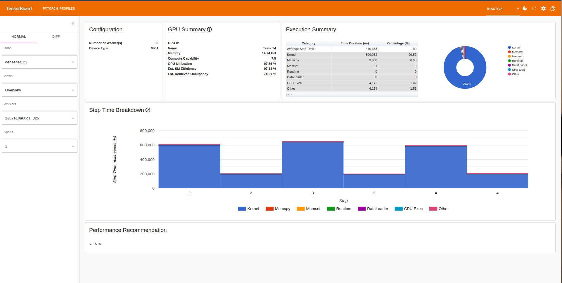
To see how the model uses memory we can head over to the memory section in tensorbard which shows mmemory usage over time. Some of the components are as follows:
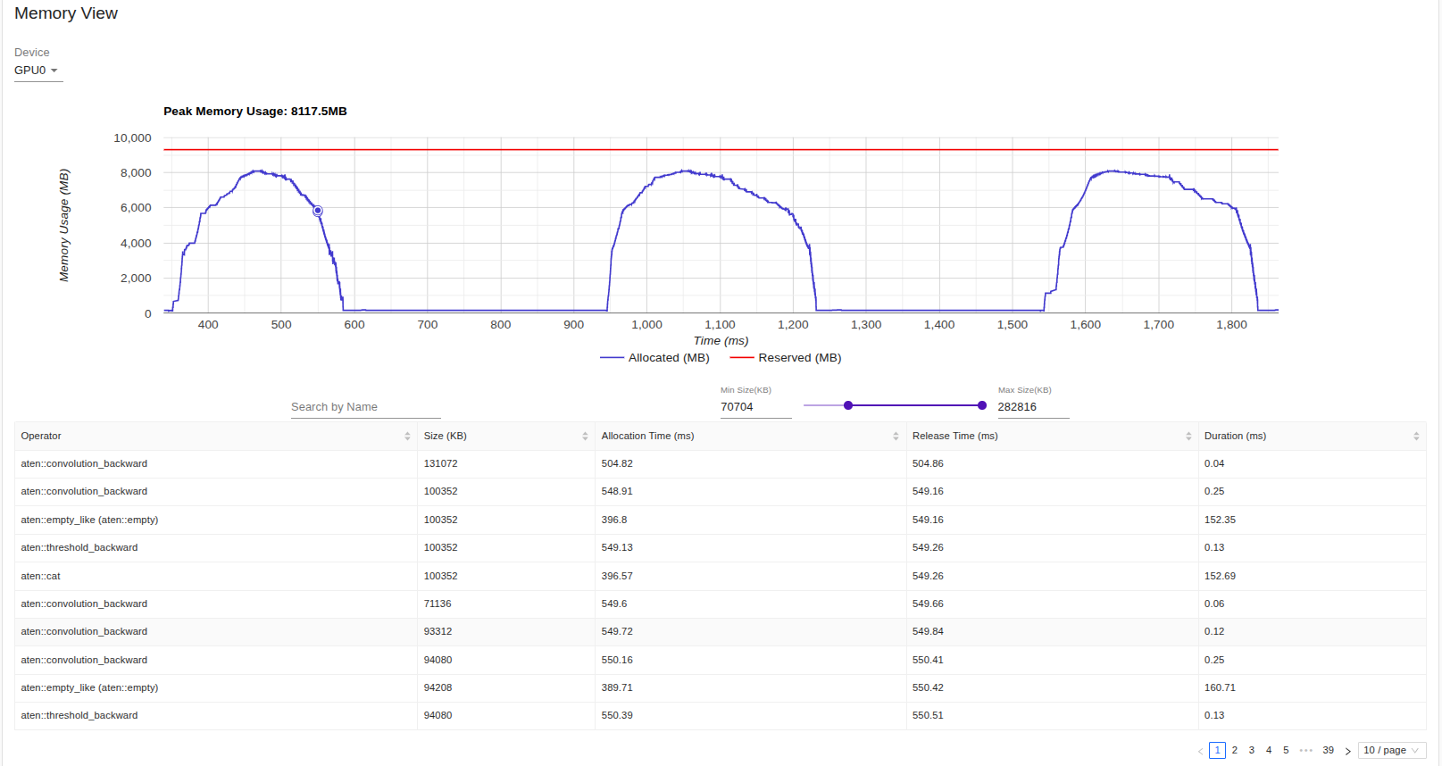
- Memmory Usage Over Time: A timeline plot of memory allocations (e.g., GPU/TPU/CPU) while training or running inference.
- Breakdown by Operations: Lets you see how much memory each operation or layer in your model is using.
- Peak Memmory Usage: Shows the maximum allocated memory and reserved memmory on device.

The above image is from the kernel section, from which we can see that Tensor Cores Utilization is at 0.0% This happens due to training on FP32, hence kernels dont get mapped to Tensor Cores.
Tensor Cores usually help to accelerate matrix multiplication and accumulate operations, hence providing speedups in throughput, not using Tensor Cores results in higher precision but increased/slower training and inference and also increased memory usage.
Optimizations
Automatic Mix Precision:It’s a PyTorch feature (torch.cuda.amp) that allows your model to automatically use a mix of FP16 (half precision) and FP32 (single precision) floating-point types during training or inference.
- FP32 = 32-bit floating point (standard precision, accurate but slower, more memory).
- FP16 = 16-bit floating point (lower precision, faster, uses less memory).
It serializes PyTorch models into static, optimized computation graph that can run independently of Python
- Operator Fusion:Combines multiple operators like Conv -> BatchNorm -> ReLu into a single operation, this saves kernel from multiple executions.
- Static Graph ExecutionUnlike eager model (line by line execution in python), TorchScript runs as a compiled graph, which eliminates python overhead.
- JIT CompliationJust in time compiler rewrites and optimizes operations before execution, it can simplify expressions and remove dead code.
Open Neural Network Exchange is an open standard to represent ML models in a framework-agnostic way and ORX is ONNX Runtime which is a high inference engine got ONNX models. It has optimizations liek graph fusion, quantizations and execution providers to make inference faster than plain PyTorch in many cases.
Results from my Experiment:
The following section highlights some of the key findings from my experiments. Please note that these results were obtained on my personal machine, which has limited GPU capacity. As a result, both the batch size and number of iterations were kept relatively small—primarily to illustrate clear performance differences rather than to achieve state-of-the-art benchmarks.
The metrics recorded during this experiment include: (You can find the code here)
metrics = {
        "variant": variant_name, # variants for this experiment [baseline, amp, torchscipt, onnx-ort]
        "batch_size": dataloader.batch_size,
        "device": str(device),
        "latency_ms": avg_latency_ms,
        "median_latency_ms": med_latency_ms,
        "std_latency_ms": std_latency_ms,
        "throughput_samples_sec": throughput,
        "cpu_time_total_ms": cpu_time_total_ms,
        "cuda_time_total_ms": cuda_time_total_ms,
        "ram_usage_mb": None,  # torch.profiler gives op-level CPU mem; we leave None (PyTorch kernel-only)
        "vram_usage_mb": None,  # not directly aggregated by profiler; peak_allocated_mb is provided
        "peak_memory_allocated_mb": peak_allocated_mb,
        "peak_memory_reserved_mb": peak_reserved_mb,
        "cpu_utilization_pct": cpu_util_pct,
        "gpu_utilization_pct": gpu_util_pct,
    }
We benchmarked DenseNet121 on CIFAR-10 using different optimization techniques: baseline (FP32), AMP autocast, TorchScript, and ONNX Runtime.
- AMP autocast achieved the lowest latency (~418 ms) and highest throughput (~38 samples/sec), showing clear gains in efficiency with minimal accuracy change.
- TorchScript offered a modest speedup compared to baseline but had higher model load overhead (~37 s).
- ONNX Runtime produced the slowest inference (~978 ms latency) and lowest throughput, indicating suboptimal backend support for this setup.
- Accuracy remained consistent across optimizations (~12.5% top-1, ~62.5% top-5), which is expected given the model was re-purposed from ImageNet to CIFAR-10 without full retraining.
| Method | Batch | Device | Latency (ms) | Throughput (sps) | Top-1 Accuracy |
|---|---|---|---|---|---|
| baseline | 16 | cuda | 578.58 | 27.65 | 12.5 |
| amp_autocast | 16 | cuda | 418.49 | 38.23 | 12.5 |
| torchscript | 16 | cuda | 634.74 | 25.21 | 12.5 |
| onnx_ort | 16 | cuda | 978.53 | 16.35 | None |